DEEPCRAFT™ Siren Detection Ready Model Report
In this document, we describe the DEEPCRAFT™ Ready Model for Siren Detection, an audio-based AI model developed by Imagimob, an Infineon Technologies company, that detects sirens from emergency vehicles. We provide details about the technical specifications of this machine learning model, its performance in common scenarios, and various test results for the model including the real-time testing on an Infineon PSOC™ 6 board.
All recommendations, performance information, and other details mentioned in this report refer exclusively to the Ready Model included in the project. Any modification to the model — such as retraining, altering its architecture, or changing its parameters — is likely to invalidate these details, including the stated recommendations and performance metrics.
Model specifications
Model Overview
The DEEPCRAFT™ Ready Model for Siren Detection detects the presence of a siren, regardless of the emergency vehicle type, such as a police car, ambulance, or fire truck. The model is trained on data from standard emergency vehicle sirens from different countries, including the U.S. To increase the robustness of the model, we used a wide range of indoor and outdoor negative sounds. The model is trained using DEEPCRAFT™ Studio and is designed to operate on Infineon PSOC™ 6 hardware with the IoT sense expansion kit (CY8CKIT-028-SENSE).
A possible use case is to switch off the noise canceling function in headphones when an emergency vehicle approaches, so that the user becomes attentive both for their own safety and to be able to leave space for the vehicle. The target group of this model is pedestrians only. Even though such a model is applicable in the automotive sector to inform drivers of upcoming emergency vehicles, deploying the model in the automotive sector poses significant challenges and is therefore out of the scope of this version.
Expected Performance
The model is expected to detect sirens from standard emergency vehicles, such as police cars, ambulances and fire trucks. Prominent sirens, that is, sirens that go on for at least a few seconds at a sufficient volume (RMS value higher than -20), are detected with rates of up to 92%. Distant or very short siren sounds may not be detected; for the intended use case it is enough to capture them when the vehicle comes closer. A siren event, compared to its background, needs to have a Signal To Noise Ratio (SNR) of at least 10 decibels (dB) in order to be detected.
During field testing with an ambulance and a fire truck in Stockholm, Sweden, the model achieved approximately 80% recall for siren events in the reported test conditions. When the emergency vehicle is at a longer distance or enables the siren for a very short period of time, the model achieves lower recall.
Detailed results are provided in Appendix I - Detailed Validation Set Results and Appendix II - Detailed Field Test Results.
Operations
The model detects any siren in its vicinity, regardless of the emergency vehicle type. The model does not trigger on every single prediction timestep during a siren; short gaps of a few seconds may occur where predictions do not pass the post-processing policy. For use cases like disabling noise cancellation, it is recommended to apply a cooldown period of a few seconds after each detection so that short gaps do not interrupt the feature. The most difficult false positives to avoid are various alarms, which are not necessarily harmful to become aware of in the intended use case, and whistling. For environments with siren-like machine sounds (such as a circular saw), it should be possible to toggle the feature off.
Model Tech Specs and Deployment
The DEEPCRAFT™ Ready Model for Siren Detection consists of several convolutional neural networks (CNNs) that capture the information from the input data features. The input data are the Fourier transformation of the audio waveform within a window of 500 milliseconds. In particular, we collect all the audio samples for 500 milliseconds, extract the Fourier transformation features, and provide the features to the model to predict the presence of a siren.
Sample rate: 16000 Hz Channels: 1 (Mono) Bit Depth: 16bit
| Target board | Model version | library - Flash (KiB) | library - RAM (KiB) | ml-middleware - Flash (KiB) | ml-middleware - RAM (KiB) | tflite-micro - Flash (KiB) | tflite-micro - RAM (KiB) |
|---|---|---|---|---|---|---|---|
| Any | ANSI C99 | 48.79 | 54.94 | N/A | N/A | N/A | N/A |
| PSOC™ 6 | float32 | 55.12 | 161.88 | 3.14 | 4.52 | 258.69 | 0.09 |
| PSOC™ 6 | int8x8 | N/A | N/A | N/A | N/A | N/A | N/A |
| PSOC™ Edge | float32 | 165.63 | 161.90 | 4.27 | 4.62 | 264.32 | 0.12 |
| PSOC™ Edge | int8x8 | N/A | N/A | N/A | N/A | N/A | N/A |
Memory-footprint calculation details are provided in Appendix IV - Memory Footprint Calculation.
For on-device testing and inference time calculation, the model uses generic C99 code containing the float32 model implementation and its preprocessing. It does not require a separate ML runtime. The inference time is about 20 ms when running on a PSOC™ 6 (model CY8CKIT-062S2-43012) overclocked to 150 MHz and mounting an IoT Sense expansion kit (model CY8CKIT-028-SENSE). The model outputs a prediction every 512 ms.
Dataset
Positive Data
The positive data includes siren sounds from fire trucks, ambulances, and police vehicles, with a focus on U.S. sirens while also including sirens from other countries. The recordings cover different siren types, background noises, and distances.
There are three primary siren sounds we’ve focused on that seem to capture the vehicles of interest. As shown in Figure 1, the three siren sounds can be characterized in the frequency domain as follows:
- Slow sine pitch alternation
- Square-formed pitch alternation
- Fast sine pitch alternation
Examples from a spectrogram plot:
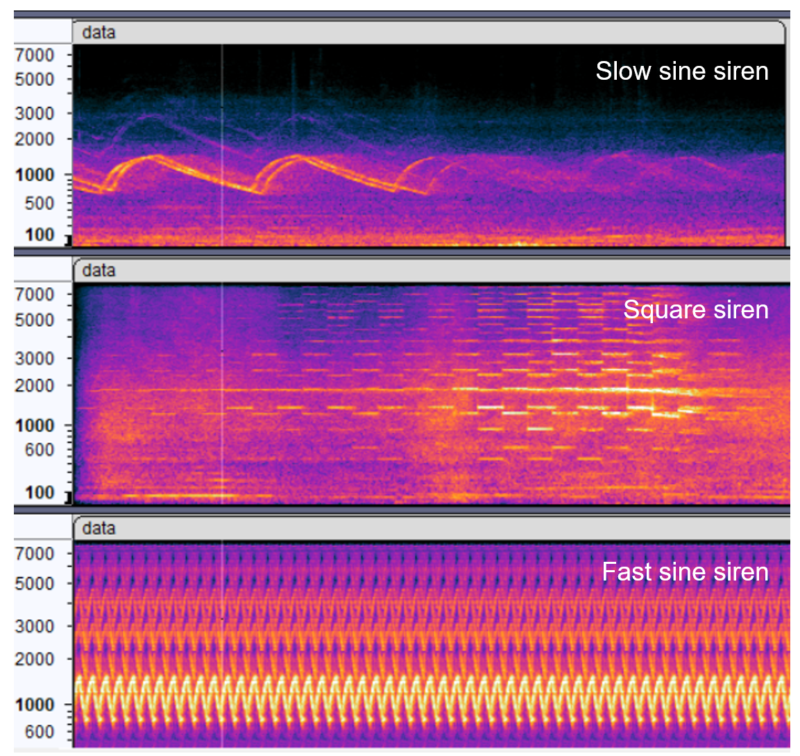
Figure 1 Spectrogram plots for the three main frequency domains
Negative Data
The model has also been trained and tested on various negative indoor and outdoor sounds. Special care has been taken to:
Not trigger false positives on sounds that occur in situations where the user would not want noise canceling to be interrupted, such as flight cabins, public transport, various machinery like drills and saws, etc. Focus on sounds, other than sirens, that also alternate or move across pitch, such as string trimmer, circular saw, electric shaver, cat meowing, etc. Below is a representative, non-exhaustive list of prominent negative sound categories validated against. Some categories, such as “public transport”, are broad and contain a range of sounds. Siren recordings also contain background sounds from their natural environments that are not listed separately.
- Alarm bell
- Bells
- Birds
- Blender
- Car horns
- Cat
- Chainsaw
- Children playing
- Church bells
- Circular saw
- Crowd
- Dinner
- Dog
- Doorbell
- Drill
- Electric shaver
- Electric toothbrush
- Elevator tone
- Firework
- Flight takeoff and landing
- Footsteps
- Keyboard typing
- Kitchen machines
- Laughter
- Leaf blower
- Melodies blended with background sounds like traffic
- Music
- Ocean waves
- Office
- Phone alarms
- Public transport
- Rain
- Scooter engine
- Speech
- String trimmer
- Thunderstorm
- Traffic noise
- Train passing
- TV and radio broadcast
- Vacuum cleaner
- Various alarm bells
- Vehicle engine
- Water dripping
- Whistling
- Wind
- Wood chopping
Model Evaluation
In this section we present the evaluation of the model. The model was evaluated in two ways, each described in one of the following subsections:
- Validation set results: performance on realistic sound data not used during model training, evaluated in DEEPCRAFT™ Studio.
- Field test results: real-time performance with the model deployed on-device, tested with a real ambulance and fire truck in Stockholm, Sweden.
- Field test results: real-time performance with the model deployed on-device, tested with a real ambulance and fire truck in Stockholm, Sweden.
We evaluate model performance at two levels: file level and sliding-window level. At file level, each sound file counts as one result: a positive file is classified as detected if the model triggers at least once anywhere in the file, and a negative file is classified as a false positive if the model triggers at least once anywhere in the file. At sliding-window level, each model input window and resulting prediction counts as one result.
Validation Set Results
For this evaluation, we extract the confusion matrix from DEEPCRAFT™ Studio on sounds not used during the model training.
Sirens were divided into more prominent sirens that were louder and closer versus less prominent ones that were further away and had lower volume. The criterion is that the siren must go on for at least a few seconds at an RMS value higher than -20. These more prominent sirens represent over 60% of the data.
Table 1 shows the confusion matrix at sliding-window level. When a positive siren input is given to the model, the model should respond with a positive value, and vice versa.
The percentages in both confusion matrices are normalised within each actual class column, so the diagonal values are recall values for the corresponding class:
- Top Left Value (Negative Recall / True-Negative Rate): actual negative data predicted as negative
- Bottom Left Value (False-Positive Rate): actual negative data predicted as positive
- Top Right Value (False-Negative Rate): actual positive data predicted as negative
- Bottom Right Value (Positive Recall / True-Positive Rate): actual positive data predicted as positive
| Sliding-Window-Based Confusion Matrix | Actual negative | Actual siren |
|---|---|---|
| Predicted negative | 92.35 % | 21.86 % |
| Predicted siren | 7.65 % | 78.14 % |
Table 1: Sliding-window level confusion matrix on the validation set.
We observe that the model correctly caught 92% of these sliding-window results as true negatives among the negative data. For the sirens, it was able to catch around 78%. It is worth noting that a share of these sirens is distant, so we would not expect the model to be able to distinguish them all too well; for the use case, it is enough to capture them when they become a bit closer.
Table 2 presents the confusion matrix on the same data at file level. The model performance is evaluated by detecting the presence of at least one positive siren prediction anywhere in the file.
| Files-Based Confusion Matrix | actual negative | actual siren |
|---|---|---|
| Predicted negative | 97.38 % (931 files) | 19.16 % (55 files) |
| Predicted siren | 2.62 % (25 files) | 80.84 % (232 files) |
Table 2: File level confusion matrix on the validation set (confidence threshold 0.75, 4 consecutive predictions).
We observe that the model triggers a false prediction event on 2.6% of the negative files while capturing a bit more than 80% of the sirens, a set that still contains siren files that are distant and/or short.
Figure 2 illustrates the percentages of triggers at file level per category. The plot shows the model can effectively capture closer sirens while suppressing triggers on various negative background sounds. This is with the default post-processing, but the customer can adjust the model’s sensitivity depending on their preference for capturing more positives or suppressing more negatives.
The most difficult false positives to avoid for the model are generally various alarms. While we significantly suppressed them, they are not necessarily harmful to become aware of, such as in the use case of shutting off noise canceling. Whistling also showed some false positives, but it is not assumed to be a significant part of someone’s everyday life.
For more detailed results in all categories, please review Appendix I - Detailed Validation Set Results.
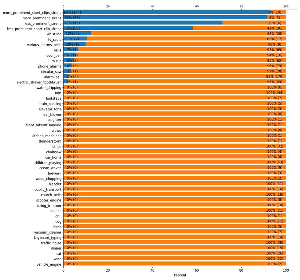
Figure 2: Histogram of model predicting that the file contains a siren versus not containing a siren.
In Figure 3 we present the false positives that triggered the model on negative sounds. We observe that if someone was constantly whistling, it would for example trigger roughly more than once per minute as a false positive. For categories like music, television and radio, these sounds are likely to be more in the foreground of the audio, which is not necessarily the case in noisy environments where they are blended with other sounds and less likely to trigger a response from the model.
There are some categories, like circular saw, which might require the ability to toggle off the feature when working in an environment where such tools are used; in such environments, however, robust hearing protection is more likely to be worn than headphones.
For more detailed results in all categories, please review Appendix I - Detailed Validation Set Results.
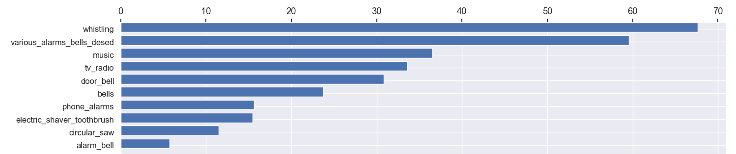
Figure 3: False positive siren event triggers per hour on negative sounds.
Field Test Results
We conducted field testing with the model deployed on-device, using a real ambulance and fire truck in Stockholm, Sweden. More details about the field testing can be found in Appendix II - Detailed Field Test Results.
- Ambulance Testing On-Device in Western Stockholm
We conducted the ambulance field testing at an ambulance station in the western parts of Stockholm. In this experiment, both the tester and the ambulance were static, and the ambulance driver was triggering the siren alarm to monitor the model reaction. We tested both the square form and fast sine form siren.
- Ambulance Drive-By
In this set of experiments, the tester was static, and the ambulance drove and passed by the tester. The purpose of this experiment is to monitor the model performance in a more realistic scenario than before, where the emergency vehicle is approaching the pedestrian. In this test, the ambulance driver had the siren activated, and it drove by the tester on the street three times. We observed that the model did indeed trigger every time, and the model continued to detect the siren at a distance notably longer than 50 meters.
- Ambulance Static and Tester Walking
In this set of experiments, the tester started close to the ambulance and then walked away. During these tests, we observed that the model triggered predictions consistently and with high confidence.
- Fire Truck Testing in Stockholm
Similarly, we conducted experiments on a fire truck. In this set of experiments, we observed results similar to the ambulance tests. It is worth noting that when the fire truck was driving further away from the tester, at distances of more than 50 meters, siren detection became less reliable.
Summary
The evaluation shows that the model detects prominent sirens reliably while suppressing false positives on a wide range of negative sounds:
- On the validation set, the model detected around 81% of the siren files (up to 92% for prominent sirens) and triggered false positives on only 2.6% of the negative files.
- In field testing with a real ambulance and fire truck, the model triggered on every ambulance drive-by; performance varied with the distance from the emergency vehicle.
- The most difficult false positives are various alarms and whistling; these can be further suppressed with post-processing depending on the use case.
Appendix I - Detailed Validation Set Results
This appendix provides detailed validation set results per sound category: the distribution of file lengths, the file level trigger histogram, the false positive triggers per hour, and the average predicted siren probability per category.
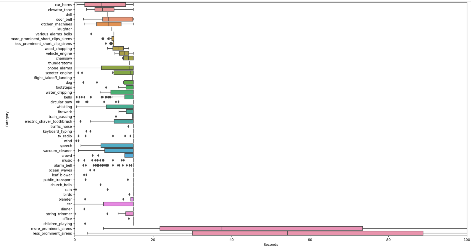
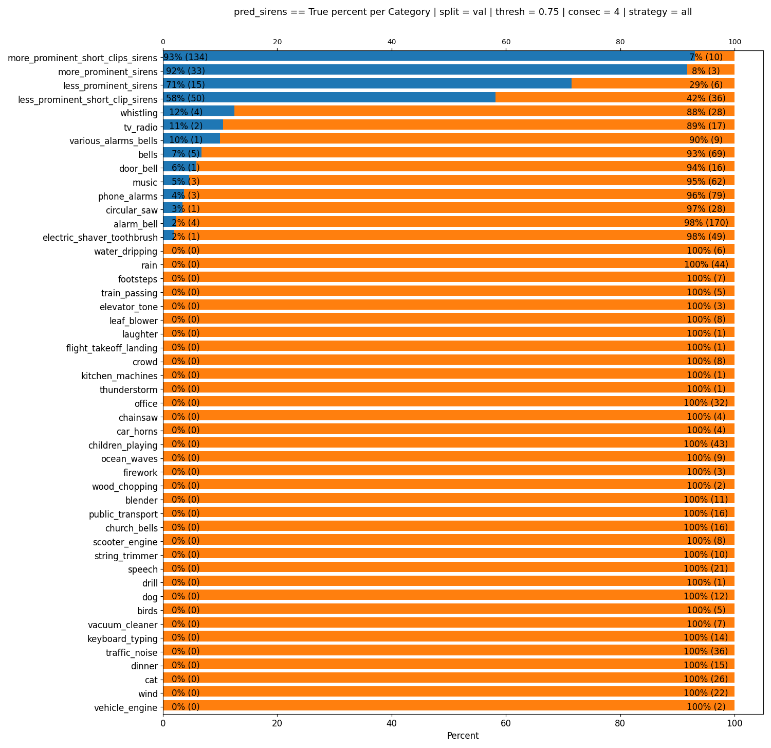
Figure 5: File level histogram of model predicting that the file contains a siren versus not containing a siren.
Notes for this plot:
- The percentages mean how many triggers there are at file level (given the post-processing).
- The values in parentheses after the percentages on the bars show how many files the percentage represents.
- The negative background sounds for the validation set have been split into 15 second file segments for a fairer comparison across categories.
The plot shows that the model can effectively capture closer sirens while suppressing triggers on a wide range of negative background sounds. This is with the default post-processing, but the customer can adjust the sensitivity of the model depending on their preference for capturing more positives or suppressing more negatives.
The hardest false positives to avoid for the model are generally various alarms, and while we significantly suppressed them, they are not necessarily harmful to become aware of, such as in the use case of shutting off noise canceling. Also, whistling has been showing some false positives, but it is not assumed to be a major part of someone’s everyday life.
False Positive Triggers per Hour on Negative Background Data
Another way to evaluate the results is to simulate how many false positives the model would trigger on the negative background categories per hour. We do this by:
- Dividing this background data into 5 second chunks, as a proxy for counting “annoyances” for a user being nudged by a false positive.
- Evaluating if the model would have triggered a siren prediction for each chunk given the default post-processing (only counting maximum one trigger per 5 second window).
- Calculating the ratio of total number of triggered siren events per hour.
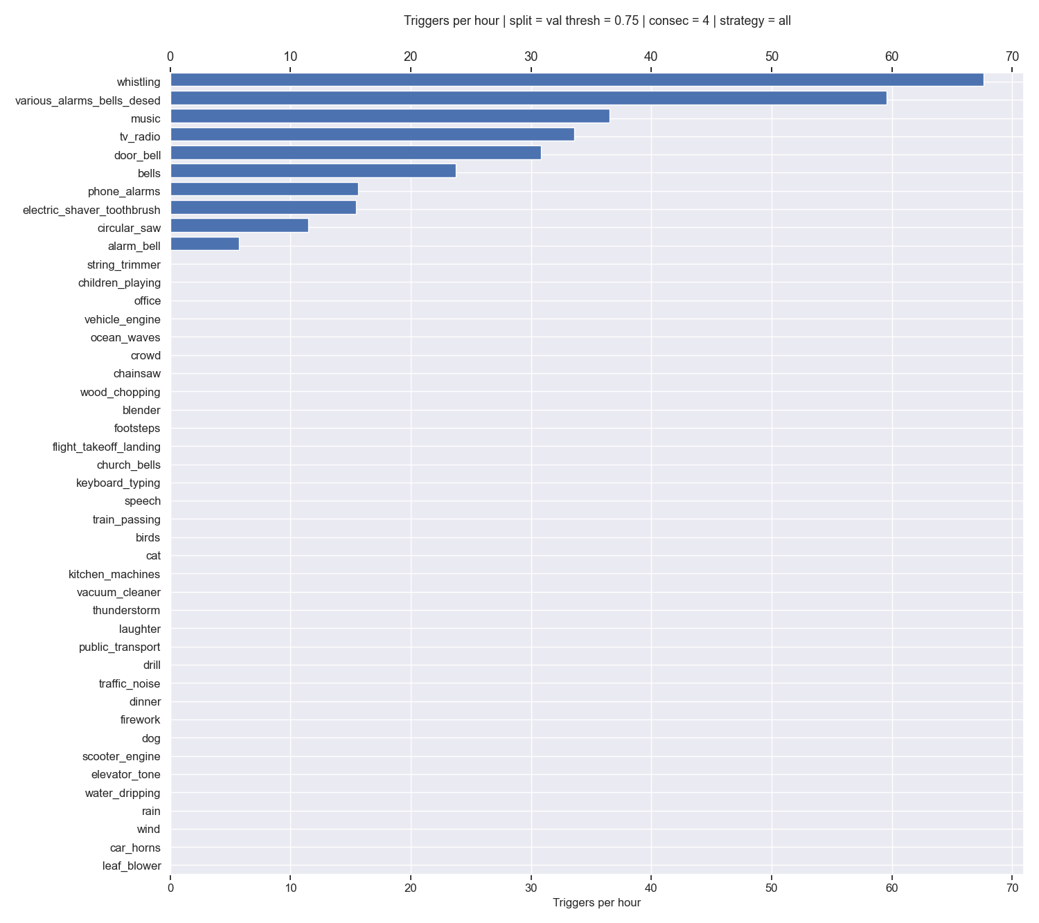
Figure 6: False positive siren event triggers per hour on negative sounds.
What we can see here is that if someone was constantly whistling, it would for example trigger roughly more than once per minute as a false positive. For categories like music, television and radio, these sounds are likely to be more in the foreground of the audio, which is not necessarily the case in noisy environments where they are blended with other sounds and less likely to trigger a response from the model.
There are some categories, like circular saw, which might require the ability to toggle off the feature when working in an environment where such tools are used; in such environments, however, robust hearing protection is more likely to be worn than headphones.
Note once again that we effectively suppress several sounds completely from triggering in the validation set.
Average Predicted Siren Probability per Negative Category
Lastly, another way to evaluate the results is to look at what the model predicts on average across all sliding windows for each category. This is sometimes also called the confidence of the model that a data point belongs to a certain class (here: sirens). Stated differently, this means what the model thinks the probability of a given data point being a siren is. For negative classes we want these probabilities to be as low as possible, showing that the model is not reacting to them.
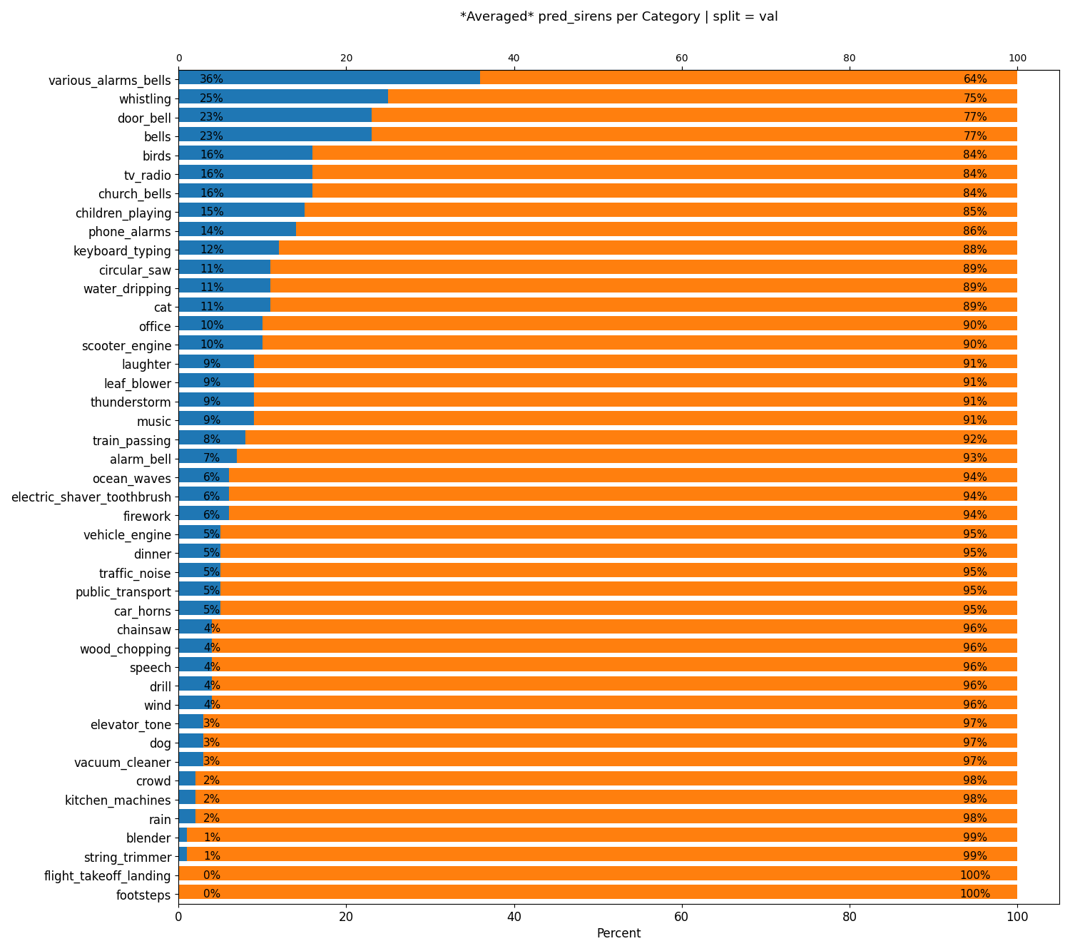
Figure 7: Average predicted siren probability for sounds across samples per category.
We can see here that the model averages very low probabilities for several sounds, which supports that we do not need to be too concerned about false positives for those (like drills, speech, kitchen machines, flight takeoff and landing, etc.).
Other Considerations for False Positives
An even more effective way of suppressing false positives for contexts other than a pedestrian walking down a street would be to toggle the model on/off based on some intelligent feature such as GPS location change. Then it could be switched off from triggering any false positives when the user is staying at home or at work, and come online again once the person is walking down a street.
Appendix II - Detailed Field Test Results
Model triggering siren event when siren approaches from the distance:
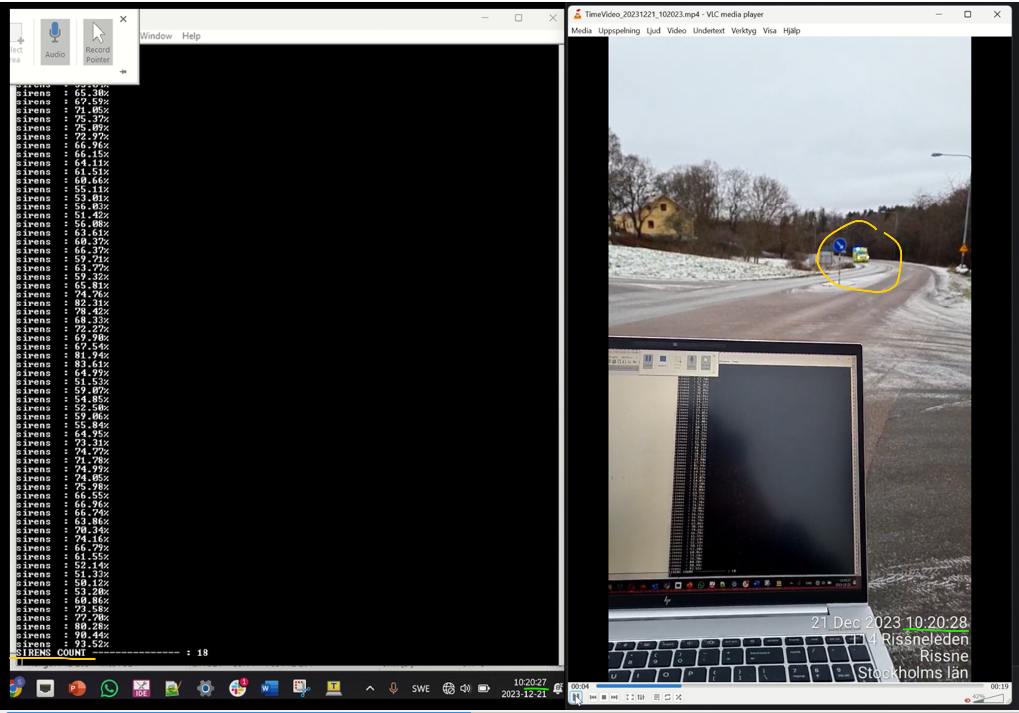
Figure 8: Model triggering siren event when the siren approaches from the distance.
Model continuing to trigger siren events as the ambulance approaches:
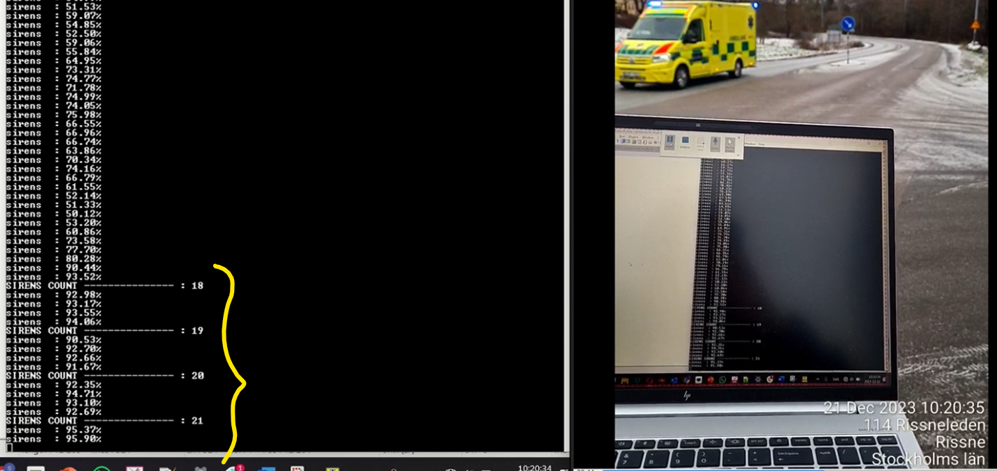
Figure 9: Model continuing to trigger siren events as the ambulance approaches.
We did note that the model, in one of the three drives, using the post-processing filtering, missed some seconds when the vehicle was getting closer and swapping to the fast sine wave form (which is usually not a problem). It did however catch the siren initially. In the use case of fading out music and removing noise canceling in headphones, it would still have worked well if the feature had a cooldown period of a few seconds, and the user would still have become attentive based on the two initial event triggers when the ambulance approaches in the far end of the curve in the picture.
Ambulance Standstill and Varying Distance by Walking
In these tests we started close to the ambulance and then walked away. The model triggered predictions consistently and with high confidence.
We do note once again that it can happen for a few seconds that the predictions do not get past the post-processing policy and therefore would not trigger the feature for those time steps.
Square form siren
In the first screenshot, walking away from the vehicle, the siren event triggers on around 80% of the occasions (11 / (11 + 3)) where the post-processing is successfully passed, with a gap in the end.
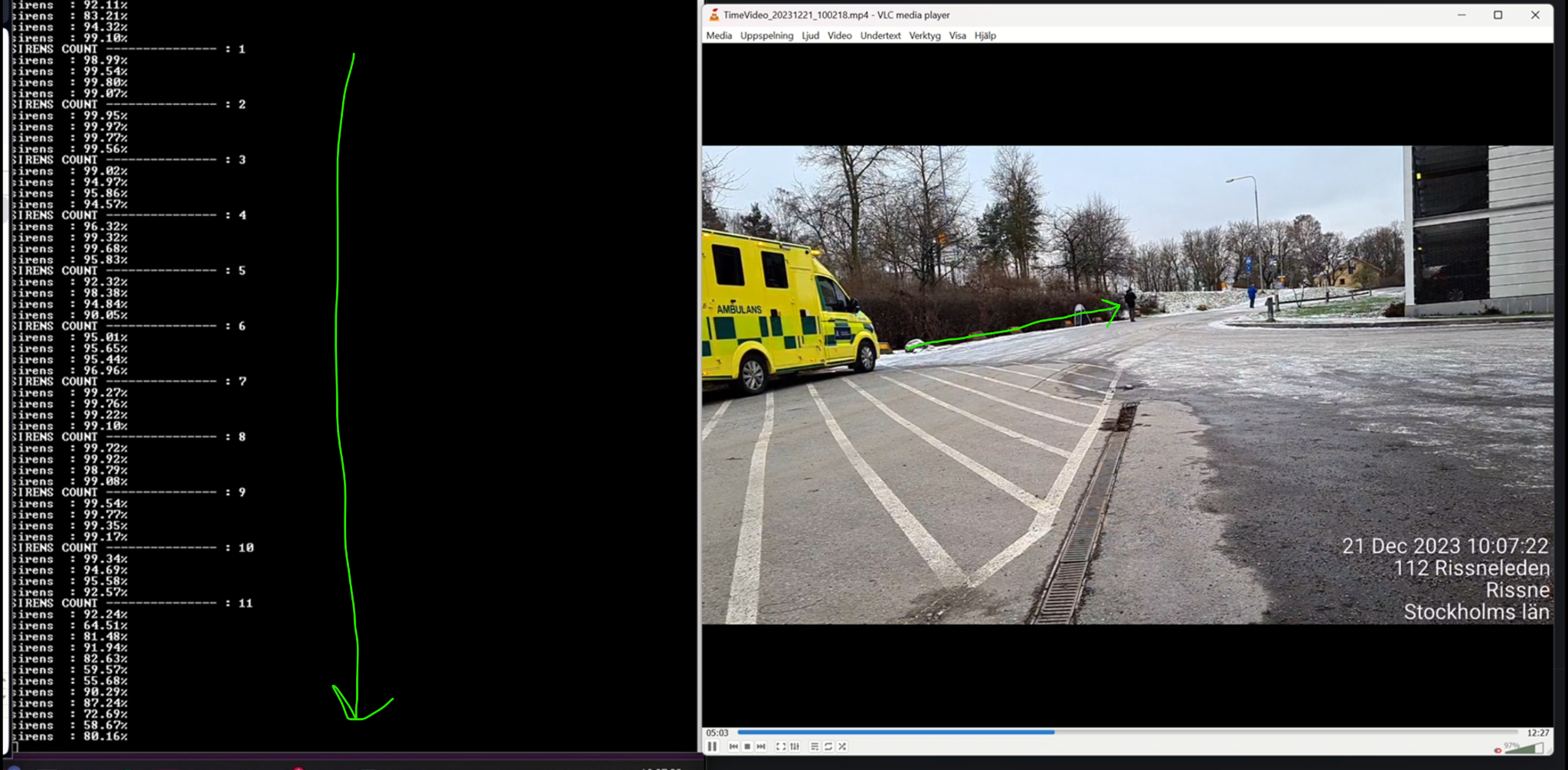
Figure 10: Square form siren, walking away from the vehicle.
In the next picture, at around 80 m distance from the vehicle, the model captures around two thirds of the events (10 / (10 + 5)).
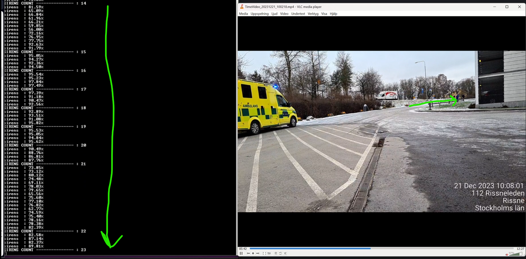
Figure 11: Square form siren at around 80 m distance.
Lastly, when standing at around 90-100 m distance (a bit further behind the building in the picture), the model overall did reasonably well. It did have some gaps but overall triggered around 75% of the time past the post-processing, which supports that we can capture vehicles in time as they approach from a distance.
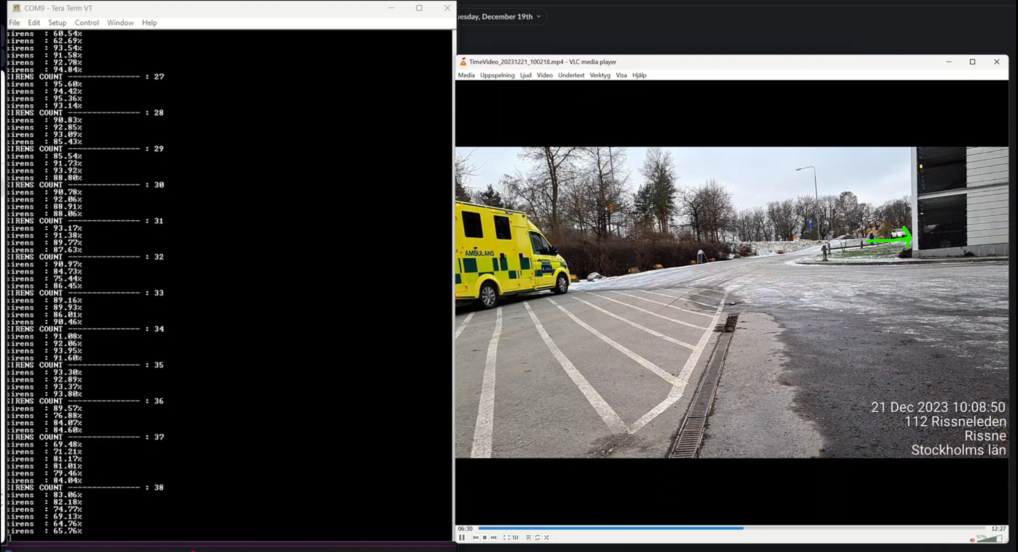
Figure 12: Square form siren at around 90-100 m distance.
Square Form Mixed with Fast Sine Siren
This test is similar to the previous test but mixes the square-formed sirens with the fast sine sirens.
From the first walking distance we can see that despite alternating so there were 2 fast sine and 2 square siren sounds, the model only missed passing one step through the post-processing (92% recall).
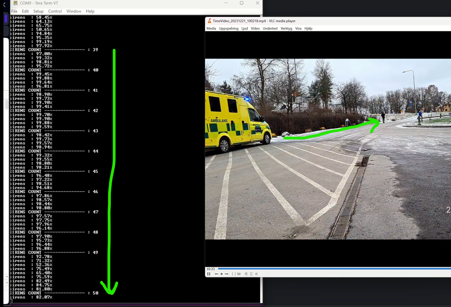
Figure 13: Mixed square form and fast sine sirens, first walking distance.
For this next section which, it should be noted, is at a longer distance, the model had one gap that was a bit longer, over several seconds, containing mostly the fast sine siren. The model did however infer above 70% probability for many of these time steps, and caught 4+ consecutive events passing the post-processing both before and after this gap.
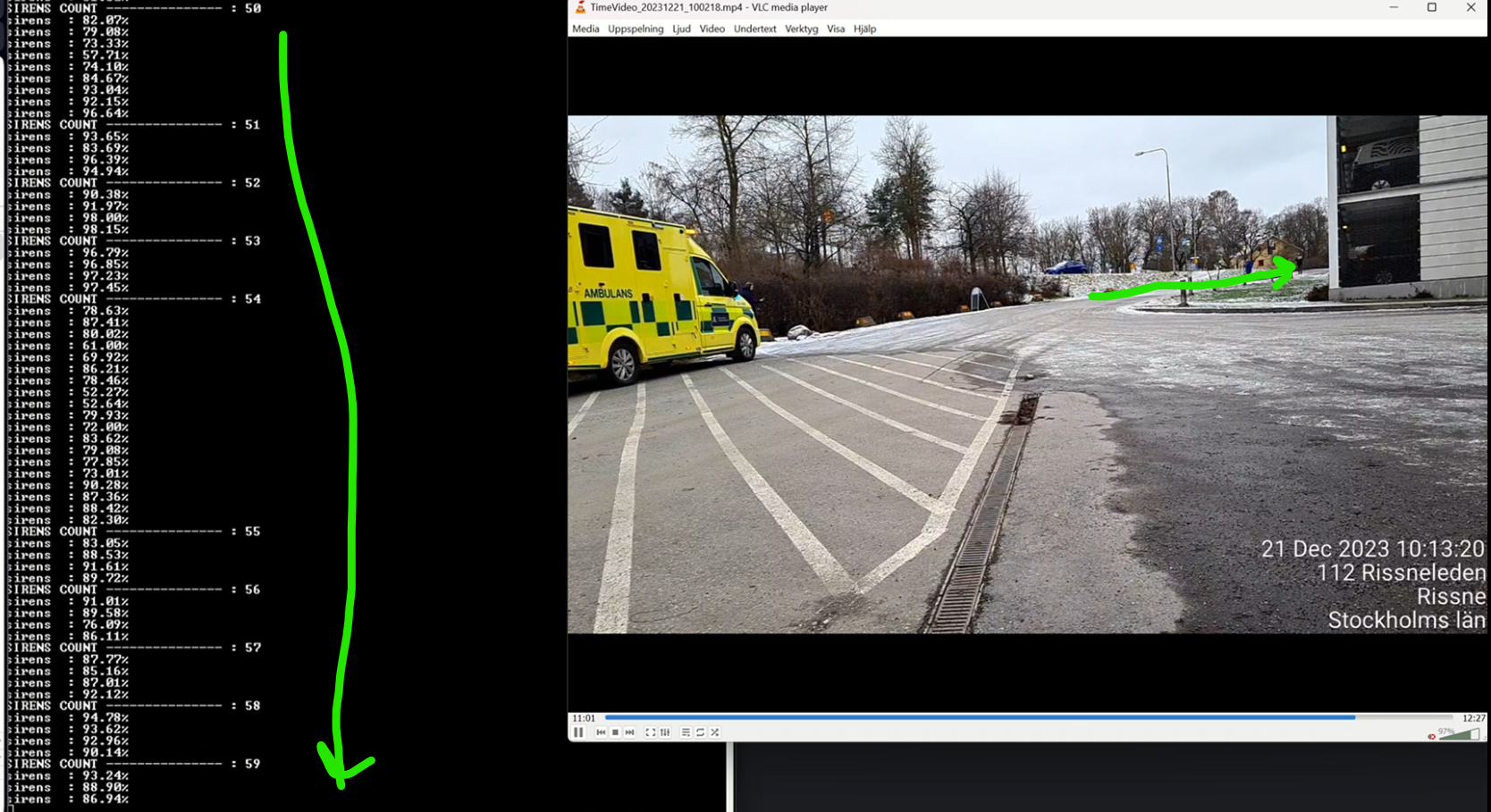
Figure 14: Mixed square form and fast sine sirens, longer distance.
Final remarks on static ambulance tests
One thing to note is that the natural state of emergency vehicles is to be in a hurry, not standing still for many seconds. It could be that the model finds it easier to identify the real approaching siren because it has learnt that there should in most cases be some slight Doppler effect, as it is common that the vehicles are on the move.
Fire Truck Testing in Stockholm
Similar testing was performed on a fire truck. Here it can be seen that when the fire truck was close by, multiple detections were triggered, 18 in total for the same fire truck, but as it went further away the model was unable to successfully detect it.
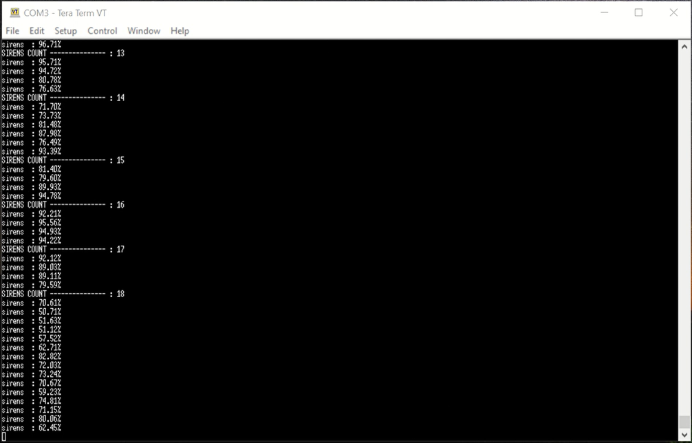
Figure 15: Fire truck testing in Stockholm.
Appendix III - Data Sources
Model data was downloaded from: Freesound and DESED
The datasets are licensed under a combination of CC0 1.0, CC BY 3.0, and CC BY 4.0.
Appendix IV - Memory Footprint Calculation
All memory values in the deployment table are KiB, where 1 KiB = 1024 bytes. Memory usage was measured by building the audio deployment examples with the GCC_ARM 14.2.1 compiler and its Debug configuration flags, then analyzing the generated linker map, as the examples existed on September 4, 2026:
The calculation parses the Linker script and memory map portion of the GNU linker map. Each input section is attributed to the generated model object, TensorFlow Lite for Microcontrollers (libtensorflow-microlite.a), or ML Middleware (libraries_shared/ml-middleware). The size reported for each input section is then added to the Flash and/or RAM total for its component according to its enclosing output section.
For PSOC™ 6, Flash is the sum of .text + .rodata + .data, and RAM is the sum of .data + .bss + .noinit. For PSOC™ Edge, Flash is the sum of .app_code_main + .app_code_itcm + .app_code_socmem + .ram_vectors + .cy_socmem_data + .data, and RAM is the sum of .app_code_itcm + .app_code_socmem + .ram_vectors + .cy_socmem_data + .data + .bss + .noinit + .cy_sharedmem. Sections that are stored in Flash and executed or initialized in RAM are counted in both totals. Consequently, these results describe the linked deployment example rather than a platform-independent measurement of the model alone.
The PSOC™ Edge Flash figures are currently overestimated because of a known bug in the code examples. A fix is work in progress, so the PSOC™ Edge Flash values should be treated as provisional until the corrected examples are available.