Training Object Detection Model

This section explains how to train a Object Detection model on your custom dataset using the Ultralytics YOLO model in DEEPCRAFT™ Studio.

Understanding the YOLO Model

YOLO (You Only Look Once) is a state-of-the-art object detection algorithm known for the exceptional speed and accuracy. Unlike earlier methods such as sliding window approaches or region-based models like R-CNN, Fast R-CNN, and Faster R-CNN, YOLO redefined object detection by treating it as a single regression problem. Introduced in 2015, it enabled real-time detection by predicting object classes and bounding boxes in one unified pass through a convolutional neural network (CNN). YOLO divides an image into a grid, with each cell responsible for detecting objects within its region. It makes multiple predictions per cell and filters out low-confidence results, ensuring efficient and accurate detection. This architecture allows YOLO to perform exceptionally well in real-time applications across various domains.

YOLO models come in multiple variants — Nano, Small, Medium, Large and Extra Large, each optimized for different performance and resource requirements. The YOLO Nano model, supported in DEEPCRAFT™ Studio, is the smallest and most lightweight variant (YOLOv5n and YOLOv8n). Designed for edge devices and low-power environments, these models offer fast inference speeds with minimal computational overhead. For instance, YOLOv5n achieves inference in approximately 73.6ms on CPU with 1.9 million parameters, making it suitable for applications where speed and efficiency are prioritized over maximum accuracy

For more details, refer to the Ultralytics official documentation (opens in a new tab).

How to train your Object Detection Model?

Training the Object Detection model using the YOLO framework is straightforward and intuitive. Below are the steps you need to follow to train your model:

1. Select the YOLO Model and set the Training parameters
2. Set Augmentation and Advanced Training parameters (optional)
3. Start and track the Training Job
4. Download the Model and Model Predictions

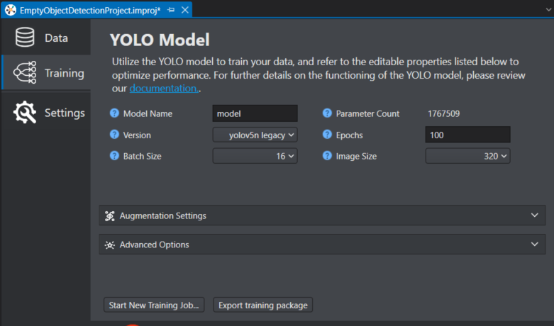
Select the YOLO Model and set the Training parameters

1. In Model Name, enter the name you want to assign to your model.

2. In Version, select the YOLO architecture you want to use for training your object detection model on your custom data. You can select from the following: YOLOv5n or YOLOv8n.

   • YOLOv5n (opens in a new tab) is known for the exceptional speed, ease of use, and mature ecosystem. It uses an anchor-based approach and is optimized for real-time object detection, making it suitable for edge devices and rapid prototyping. YOLOv5 is widely adopted due to its simple API, extensive documentation, and support for various model sizes.

   • YOLOv8n (opens in a new tab) is a versatile model that introduced architectural improvements such as an anchor-free detection head and supports multiple vision tasks including detection, segmentation, classification, and pose estimation. It offers an optimal balance between speed and accuracy, features a user-friendly design, and is well-suited for a wide range of real-world deployment scenarios.

   To compare and know about the different YOLO models, refer to Models Supported by Ultralytics (opens in a new tab).

   
   
   

3. In Batch Size, select the number of training samples to be processed in a single iteration during model training. Instead of processing the entire dataset at once, the data is divided into smaller groups called batches for efficiency and scalability, especially when working with large datasets or limited memory. After each batch is processed, the model's parameters are updated, enabling more manageable and faster training. The optimal batch size depends on the total number of training samples per window. Using larger batch sizes will speed up the completion of each epoch (full iteration over the training dataset) but will require significantly more GPU memory. On the other hand, smaller batch sizes may improve the model’s ability to generalize but can increase the training time. For instance, a batch size of 32 is generally effective for around 1000 training samples, while a batch size of 128 is more appropriate for about 5000 training samples.

4. The Parameter Count displays the number of parameters in the selected model depending on the model version and class count. While the displayed value is appropriate for reference, the actual number of parameters is calculated within the Imagimob Cloud.

5. In Epochs, enter the number of complete training cycles the model should perform over the entire dataset. An epoch represents one complete pass through the entire training data, during which the model processes each sample, makes predictions, computes errors, and updates its internal parameters to improve performance. Training requires multiple epochs to allow the model to progressively learn and refine its understanding of the data. The optimal number of epochs varies depending on the dataset and the specific task, and is usually determined through experimentation and by monitoring validation performance to avoid issues such as underfitting or overfitting.

6. In Image Size, select the target image size to be used during model training. All the input images will be automatically resized to this dimension before being passed to the model. For instance, setting the image size to 320 ensures that each image is resized so its longest side measures 640 pixels, while preserving the original aspect ratio. This resizing process is handled automatically, eliminating the need for manual adjustments to images or labels. Larger image sizes can enhance the model’s ability to detect smaller objects, but they also increase GPU memory usage and may slow down training. Therefore, it is important to choose an image size that balances detection performance with available hardware resources and the characteristics of your dataset.

Set the Augmentation and Advanced Training parameters

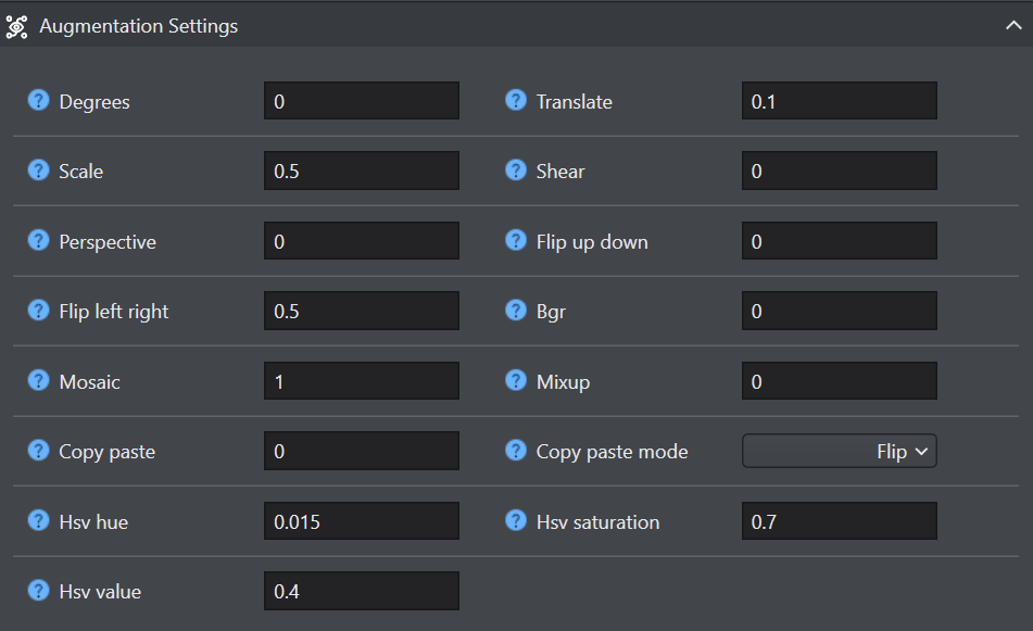
Augmentation Settings

Data augmentation techniques play a crucial role in enhancing model robustness and performance. By introducing variability into the training data, these techniques help the model generalize more effectively to unseen data. The table below details the purpose and impact of each augmentation argument:

Argument	Type	Default	Range	Description
Degree	float	0.0	0.0 - 180	Rotates the image randomly within the specified degree range, improving the ability of the model to recognize objects at various orientations.
Scale	float	0.5	>=0.0	Scales the image by a gain factor, simulating objects at different distances from the camera.
Prespective	float	0.0	0.0 - 0.001	Applies a random perspective transformation to the image, enhancing the model's ability to understand objects in 3D space.
Flip left right	float	0.5	0.0 - 1.0	Flips the image left to right with the specified probability, useful for learning symmetrical objects and increasing dataset diversity.
Mosaic	float	1.0	0.0 - 1.0	Combines four training images into one, simulating different scene compositions and object interactions. Highly effective for complex scene understanding.
Copy paste	float	0.0	0.0 - 1.0	Segmentation only. Copies and pastes objects across images to increase object instances.
Hsv hue	float	0.015	0.0 - 1.0	Adjusts the hue of the image by a fraction of the color wheel, introducing color variability. Helps the model generalize across different lighting conditions.
Hsv value	float	0.4	0.0 - 1.0	Modifies the value (brightness) of the image by a fraction, helping the model to perform well under various lighting conditions.
Translate	float	0.1	0.0 - 1.0	Translates the image horizontally and vertically by a fraction of the image size, aiding in learning to detect partially visible objects.
Shear	float	0.0	-180 - +180	Shears the image by a specified degree, mimicking the effect of objects being viewed from different angles.
Flip up down	float	0.0	0.0 - 1.0	Flips the image upside down with the specified probability, increasing the data variability without affecting the object's characteristics.
Bgr	float	0.0	0.0 - 1.0	Flips the image channels from RGB to BGR with the specified probability, useful for increasing robustness to incorrect channel ordering.
Mixup	float	0.0	0.0 - 1.0	Blends two images and their labels, creating a composite image. Enhances the model's ability to generalize by introducing label noise and visual variability.
Hsv saturation	float	0.7	0.0 - 1.0	Alters the saturation of the image by a fraction, affecting the intensity of colors. Useful for simulating different environmental conditions.

Advanced Options

The advanced training settings encompass various hyperparameters and configurations used during the training process. These settings influence the model's performance, speed, and accuracy.Careful tuning and experimentation with these settings are crucial for optimizing performance.

• Optimizer: An optimizer is an algorithm designed to adjust the weights of a neural network to minimize the loss function, which quantifies the performance of the model. In simpler terms, the optimizer facilitates the model's learning process by fine-tuning its parameters to reduce errors. Selecting the appropriate optimizer is crucial as it directly impacts the speed and accuracy of the model's learning. You can also fine-tune the optimizer parameters to enhance model performance. Adjusting the learning rate determines the size of the steps taken when updating parameters. For stability, it is advisable to start with a moderate learning rate and gradually decrease it over time to improve long-term learning. Additionally, setting the momentum influences the extent to which past updates affect current updates. A common value for momentum is around 0.9, which generally provides a good balance. To know more, refer to Ultralytics Optimization Algorithm (opens in a new tab).

Refer to table below to select from the following optimizers:

Optimizer	Definition
Auto	When the optimizer is set to 'auto', the system automatically selects the most appropriate optimization algorithm based on the model configuration and the number of training iterations. This setting overrides any manually specified values for the initial learning rate and momentum.
Adam (Adaptive Moment Estimation)	Combines the benefits of SGD with momentum and RMSProp. It adjusts the learning rate for each parameter based on estimates of the first and second moments of the gradients. Adam is efficient and generally requires less tuning, making it a recommended optimizer for YOLO11. To learn more, refer to Ultralytics Adam Optimizer (opens in a new tab)
AdamW, NAdam, RAdam	AdamW, NAdam, and RAdam are additional Adam variants supported in YOLO training. You can select any of these by setting the optimizer argument to "AdamW", "NAdam", or "RAdam" in your training configuration. These optimizers affect how the model weights are updated during training, which can influence convergence speed and stability.
RMSProp (Root Mean Square Propagation)	Adjusts the learning rate for each parameter by dividing the gradient by a running average of the magnitudes of recent gradients. It helps with the vanishing gradient problem and is effective for recurrent neural networks.
SGD (Stochastic Gradient Descent)	Instead of computing the gradient over the entire dataset at each update (as in Batch Gradient Descent), SGD updates model parameters using a single sample or a small mini-batch, which makes it efficient for large datasets and deep learning tasks. Key hyperparameters for SGD include the learning rate (lr0, default 0.01) and momentum (momentum, default 0.937), both of which can be tuned for better performance.SGD is particularly effective for large-scale models and can help with faster convergence, but may be less stable (more "noisy") than some adaptive optimizers like Adam. It remains a fundamental choice in deep learning workflows for object detection and related tasks.

• Learning Rate (opens in a new tab): The learning rate is a key hyperparameter that controls the step size taken during training to adjust model parameters and minimize the loss function. An optimal learning rate allows the model to converge efficiently to a good solution. If the learning rate is too high, training can become unstable or diverge; if it's too low, training can be slow or get stuck in suboptimal solutions. For YOLO models, typical starting values are 0.01 for SGD or 0.001 for the Adam optimizer, and you can use schedulers or warmup strategies to adjust it during training. Setting the right learning rate is crucial for effective training and achieving good model performance.

  • Initial: Initial learning rate (i.e. SGD=1E-2, Adam=1E-3). Adjusting this value is crucial for the optimization process, influencing how rapidly model weights are updated.
  • Final: Final learning rate as a fraction of the initial rate = (lr0 * lrf), used in conjunction with schedulers to adjust the learning rate over time.

• Patience: Enter the number of epochs to wait for an improvement in validation metrics before halting the training. For instance, when patience is set to 50, this means training will stop if there is no improvement in validation metrics for 5 consecutive epochs. Using this method ensures the training process remains efficient and achieves optimal performance without excessive computation.

• Confidence Threshold: Enter the minimum confidence score required for a model to consider a detection as valid during inference or evaluation, not during the actual learning process. The confidence score itself represents how certain the model is about its prediction for a detected object or class, ranging from 0 to 1. Setting a confidence threshold helps filter out predictions with low certainty, which may be less reliable. During training, the model learns to predict bounding boxes and associated confidence scores, but the threshold is primarily applied when evaluating model outputs or making predictions. For example, during validation or inference, detections with confidence scores below the set threshold (such as 0.25 by default) are ignored, while those above are kept for further analysis or display.

• Momentum: Momentum is used in optimizers during training that controls how much previous gradient updates influence the current update of the model's weights. In optimizers like SGD, a common value for momentum is around 0.9, which helps to provide a good balance by accelerating the gradient descent in the relevant direction and dampening oscillations. For Adam and similar optimizers, the momentum parameter (often called beta1) plays a similar role, influencing how much past gradients affect the current update. Adjusting momentum can impact the speed and stability of convergence during training.

• Weigh Decay: Weight decay is a regularization parameter used during training to penalize large weight values in the model. It works by adding a term to the loss function that discourages the weights from growing too large, which helps prevent overfitting. The default value for weight_decay is 0.0005, and it is applied as an L2 regularization term during optimization. Adjusting this parameter can influence the generalization ability of the model, with higher values leading to stronger regularization effects.

• Iou Threshold: The IoU (Intersection over Union) is a metric used to evaluate how well the predicted bounding boxes from the model overlap with the ground truth bounding boxes in your dataset. During training, IoU is used both as a metric for evaluating model performance and within loss functions to guide the model to improve localization accuracy. A higher IoU score means the predicted box closely matches the actual object, while a lower score indicates less overlap. Typically, IoU thresholds (such as 0.5) are used to determine if a detection is considered correct during both training and evaluation.

Start and Track the Training Job

To start the training job, follow the steps below:

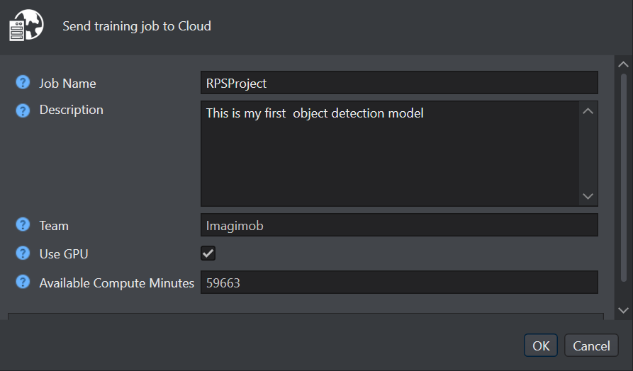
1. Click Start New Training Job to start the model training.

   
   
   

2. In Job Name and Description, enter the name of the job and description respectively.

3. In Team, the name of the team that is used for training job is displayed. If you want to use the other team, navigate to Active Team dropdown at the top right corner of studio and select the desired team.

4. In Use GPU, enable the checkbox for GPU powered training. We highly recommend utilizing the GPU for fast and efficient training.

5. In Available Compute minutes, your total credits points are displayed.

6. Click OK to begin the training. A popup window appears indicating that the job has been started. Once again click OK to view the progress of the job in a new tab.

   
   
   

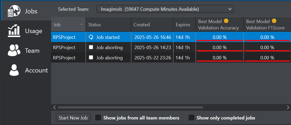
After you set the parameters for starting the model training, the model is sent to Imagimob Cloud for training. Depending on the size of the model, the training may take hours or days to complete. You can track the progress of the training jobs from Studio, whenever required.

To track the training job, follow the steps:

1. On the menu bar, click the Imagimob Cloud icon. The account portal window opens.

2. Double click the required job on the right pane to track the progress of the training job. The view updates in real time as the job progresses.

   
   
   

Download the Model and Model Predictions

After you have trained the model in Imagimob Cloud, the next step is to download the model and the predictions.

To download the model predictions, follow the steps:

1. Click Open Cloud icon to browse the training jobs on the Imagimob Cloud. The account portal window opens and the Jobs tab is selected, by default.

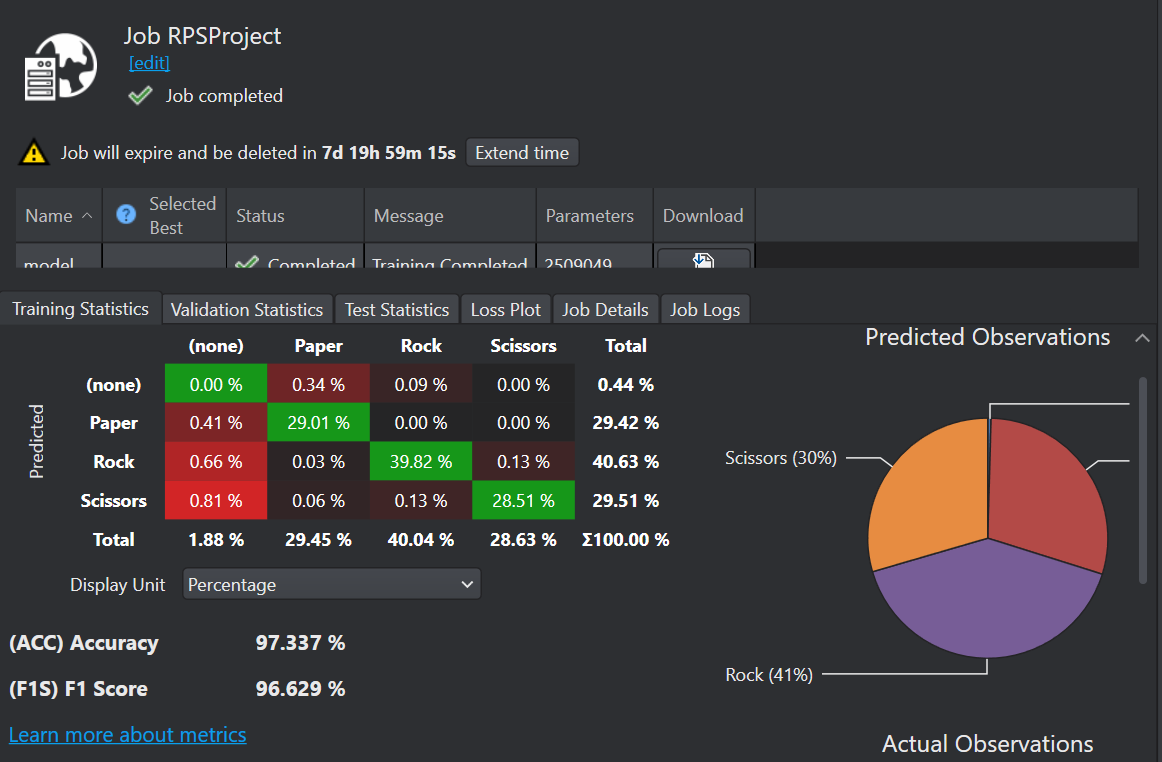
2. Double-click the training job of the project you want to track from the list of jobs. The project training job window appears in a new tab and provides the detailed view of the model.

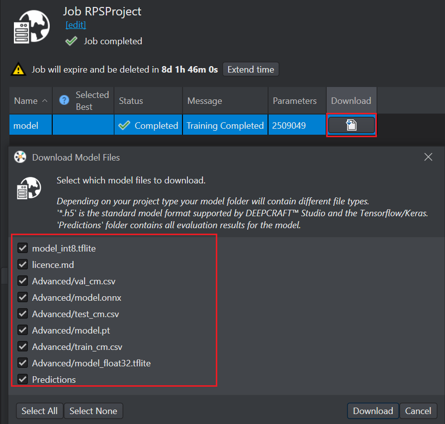
3. Scroll right to the Download column and click the Download icon to download the model predictions.

   
   
   

4. The Download model files window appears with the option to download:

   • model_int8.tflite: TensorFlow Lite model that is quantized to 8-bit integers (INT8)
   • license.md: Ultralytics YOLO License Information
   • test_cm.csv: confusion matrix files for test
   • train_cm.csv:confusion matrix files for train
   • model_float32.tflite: TensorFlow Lite model that uses 32-bit floating-point precision (FLOAT32)
   • model.onnx: model saved in ONNX format, which allows the file to be used across different platforms
   • model.pt: model saved in PyTorch's native format
   • val_cm.csv: confusion matrix files for validation
   • Predictions: model prediction files after training

5. Save the model files to an appropriate folder in your workspace. After you have downloaded the model files, the next step is to import the predictions.

After downloading the model predictions, you can add the predictions into the project to compare the bounding boxes generated by the model with the original bounding boxes in the datasets. This approach provides a comprehensive view of the model's performance. For instructions on how to import the predictions, refer to the Importing predictions into your project .

DEEPCRAFT™ Studio offers various methods to evaluate the object detection model. To know how to evaluate an object detection model, refer to Evaluating Object Detection model .