Evaluating regression model

In this section, we will explore how to use these various metrics to evaluate regression models. Assessing the performance of regression models is crucial for predicting continuous outcomes accurately. The following metrics are commonly used to evaluate regression models: R-squared (Coefficient of Determination), Mean Squared Error (MSE), Mean Absolute Error (MAE), Root Mean Squared Error (RMSE). Additionally, graphical plots tools such as Quantile - Quantile and Histogram of residuals are valuable for understanding the distribution and behavior of prediction errors. By leveraging these metrics and visualization techniques, you can effectively evaluate the accuracy and performance of their regression models.

Understanding the regression metrices and graphical plots

• R-Squared: R-Squared (R²), also referred to as the Coefficient of Determination, is a statistical metric that quantifies the proportion of variance in the dependent variable that is explained by the independent variables within a model. The value of R-squared ranges from 0 to 1, where a value of 1 signifies a model that perfectly predicts the target variable, and a value of 0 signifies a model with no predictive capability. In practical applications, the value of R-Squared typically lies between these values.

• Mean Squared Error: Mean Squared Error (MSE), also referred as L2 loss or quadratic loss, is calculated as the mean or average of the square of the difference between actual and predicted values. The lower value of Mean Squared Error implies that the model’s predictions are more aligned with the actual values, reflecting higher accuracy. On the other hand, the higher value of Mean Squared Error implies that the model’s predictions are more divergent from the actual values, indicating lower performance.

• Mean Absolute Error: Mean Absolute Error (MAE), also referred as L1 loss, is calculated as the average absolute difference between the predicted values and the actual values.

• Root Mean Square Error: Root Mean Square Error (RMSE), is calculated as the square root of mean of squared difference between the predicted values and the actual values. A smaller Root Mean Squared Error indicates a more effective model.

• Quantile - Quantile Plot: Quantile - Quantile Plot, also referred as Q-Q plot, determines whether the errors in a dataset follow a normal distribution. If the data points align along the line ( y = x ), it indicates that the errors are normally distributed. However, if the data points deviate from this straight line and form a curve, it suggests that the errors are not normally distributed, indicating that the model may not be a good fit.

• Histogram of residuals: A Histogram of Residuals plot is used to visualize the differences between observed and predicted values. One of the key assumptions in regression is that the residuals should be normally distributed. If the residuals are normally distributed, the histogram will exhibit a bell-shaped curve. If the residuals do not follow a normal distribution, it indicates potential bias in the model, suggesting that linear regression may not be the appropriate choice for the dataset.

Performing Model Evaluation of regression model

Model evaluation can be performed by following the steps below:

• Download the model files
• Import the predictions
• Evaluate the model performance using the regression metrices

After you download the model files and import the predictions, lets evaluate the model performance.

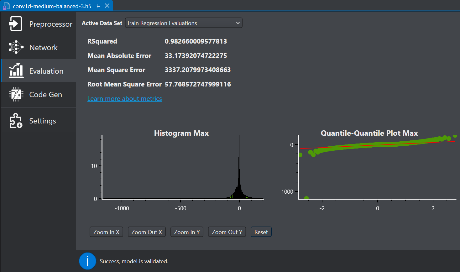
1. Navigate to your project directory and double click the *.h5 model file. The model file appears in a new tab.

2. Select Evaluation on the left pane to see an overview of the model performance. The right pane shows the various error metrics and plots which provides a summary of model predictions.

3. In Active Data Set, select the type of dataset you want to evaluate from the drop-down list. You can select Train set, Validation set, or Test set results.

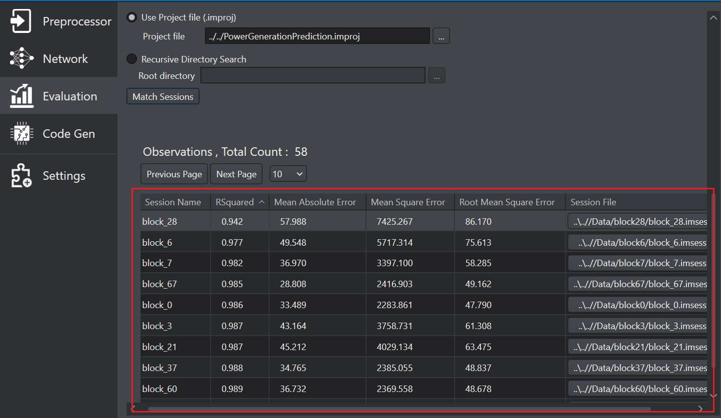
4. Configure the Representative data set parameter as per your requirement:

   • In Use Project file (.improj), select the radio button if you want to analyse the data using the project file.
   • In Project file, browse to select the project file.

   OR

   • In Recursive directory search, select the radio button if you want to analyse the data from the Data directory.
   • In Root directory, browse to select the directory.

5. Click Match Sessions to match the observations to the corresponding sessions. A popup window appears showing the match results.

   
   
   

6. Click OK to proceed. The session column in the observation list shows the sessions of the corresponding observations. You can filter the observation table in ascending and desending order and identify the sessions with maximum loss or errors.

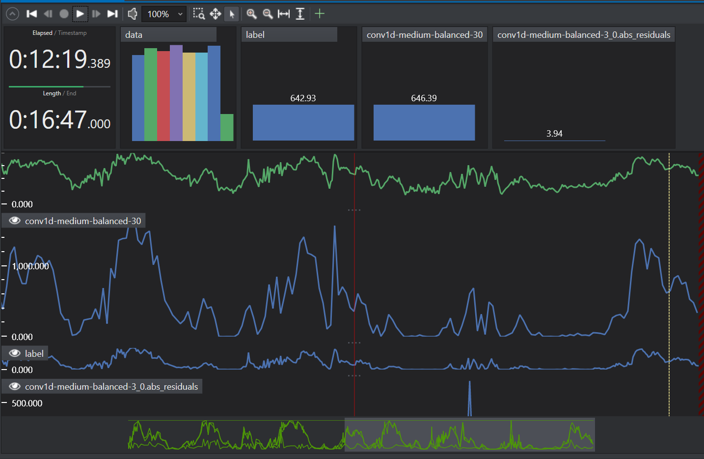
7. Click on the session under the Session File column that you want to analyze. This will provide deeper insights into the model’s performance and help you investigate the reasons behind any shortcomings.