Model evaluation using Confusion Matrix

Model evaluation is the process of using multiple statistics and metrics to analyze the performance of a trained model. You can evaluate the model performance by calculating the evaluation metrics, such as, precision, accuracy, F1 score, recall, and area under the receiver operating characteristic curve (ROC AUC) for binary classification problems and analyzing a confusion matrix for multi-class classification problems.

Understanding confusion matrix

A confusion matrix is a visual representation that summarizes the performance of a machine learning model by comparing the actual labels with the predicted labels for a set of data instances. The statistics from the confusion matrix are used to fine-tune the model so as to enhance the model performance.

Let's understand a sample confusion matrix before evaluating model performance.

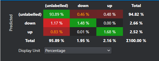
The green boxes in the diagonal represent the correct predictions and red boxes symbolize the common misprediction. All the other values outside of the diagonal is a misclassification. The rest of the metrics are standard for classification problems. To know more, refer to the documentation (opens in a new tab).

Some common terms when interpreting confusion matrix:

• True Positive: Model predicts a positive class correctly
• True Negative: Model predicts a negative class correctly
• False Positive: Model predicts a negative as a positive class
• False Negative: Model predicts a positive class as a negative class

An ideal machine learning model should have high True Positive and True Negative values while low False Positive and False Negative values. Using the above metrices, several other evaluation metrics, such as accuracy, precision, recall and F1 score can also be calculated. These metrics provides a clear summary to determine the performance of the model and highlights the areas for improvement.

Performing Model Evaluation

Model evaluation can be performed by following the steps below:

• Download the model files
• Import the predictions
• Evaluate the model performance using the confusion matrix

Downloading model files

After you have trained the model in Imagimob Cloud, the next step is to download the model files.

To download the model files, follow the steps:

1. Click Open Cloud icon to browse the training jobs on the Imagimob Cloud.
   The account portal window opens and the Jobs tab is selected, by default.

2. Double-click the training job of the project you want to track from the list of jobs. The project training job window appears in a new tab and provides the detailed view of the model.

3. Scroll right to the Download column and click the download icon to download the model files.

   
   

4. The Download model files window appears with the option to download:

   • trained model (.h5 file)
   • model predictions for evaluating the trained model
   • test input and output datasets to be used in the 'Generate Data Compare Test'

   Select the required files and click Download.

   
   

5. Save the model files to an appropriate folder in your workspace.

   After you have downloaded the model files, the next step is to import the predictions.

Importing predictions

IMAGIMOB Studio allows a much more detailed view of the performance of a model by merging the model predictions as tracks into the sessions containing the original data.

To import predictions, follow the steps:

1. Navigate to the project directory and open the project (.improj) file.

2. In the Data tab, click Add Data button.

   
   

   The Select import mode window appears.

3. Click Merge icon and browse to select the Predictions folder.

   
   

4. Select the structure of the prediction folder which is typically the Nested structure and click Next. Predictions from the selected folder will be merged as tracks into the corresponding local sessions.

   
   

5. Select or deselet what you want to import and click OK to complete the merge.

Evaluating the model performance

After you download the model files and import the predictions, you can evaluate the model performance.

To view performance statistics, follow the steps:

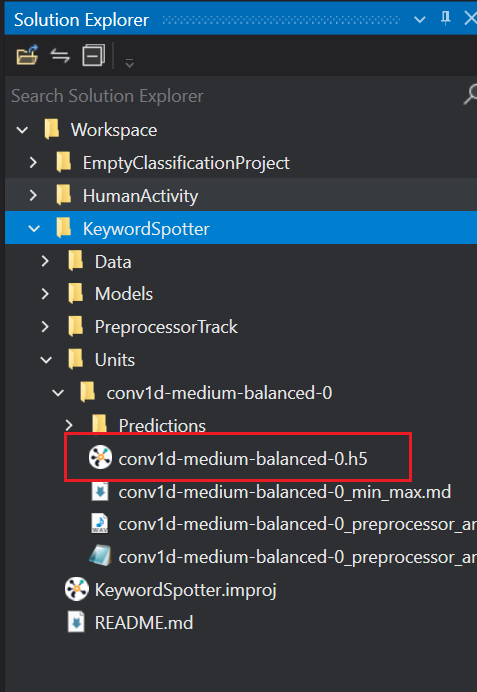
1. Navigate to your project directory and double click the *.h5 model file. The model file appears in a new tab.

   
   

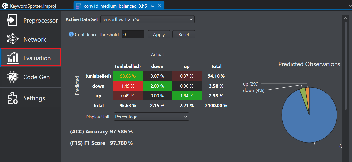
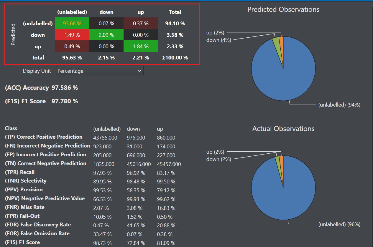
2. Select Evaluation on the left pane to see an overview of the model performance. The right pane shows the confusion matrix which provides a summary of model predictions for different activities.

   
   

3. In Active data set, select the type of dataset you want to view from the drop-down list. You can select Train set, Validation set, or Test set results.

4. In Confidence Threshold, enter the threshold value between zero and one and click Apply. The predictions that meet the confidence threshold are presented in the confusion matrix and the remaining predictions are not considered. If you do not want to filter the predictions using the confidence threshold click Reset.

5. Click on any cell in the matrix to view the cell specific obsevations in detail.

   
   

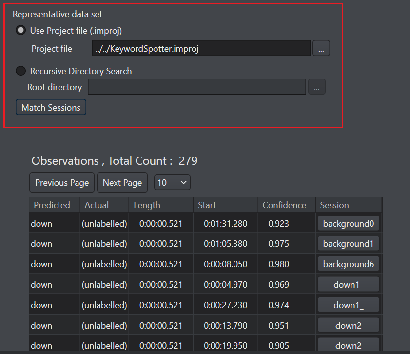
6. Configure the Representative data set parameter as per your requirement-

   
   

   • In Use Project file (.improj), select the radio button if you want to analyse the confusion matrix data against the actual data from the project file.

   • In Project file, browse to select the project file.

   OR

   • In Recursive directory search, select the radio button if you want to analyse the confusion matrix data from the Data directory.

   • In Root directory, browse to select the directory.

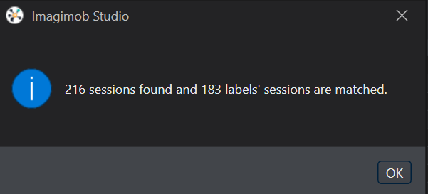
7. Click Match Sessions to match the observations to the corresponding sessions. A popup window appears showing the match results.

   
   

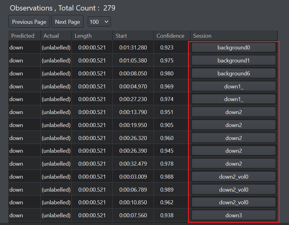
8. Click OK to proceed. The session column in the observation list shows the sessions of the corresponding observations.

   
   

9. Click the session under Session column to open and analyse the session file.

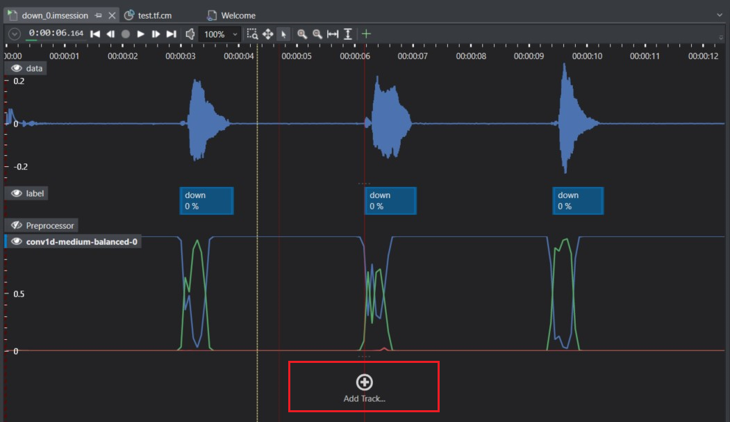
10. Click Add Track to generate a label track from predictions. This allows easy comparison of the labels predicted by the model with the actual labels set by you initially. The New Track window appears.

11. On the left pane, select Label Tracks.

12. Select Label Track from predictions from the list of options and click OK.

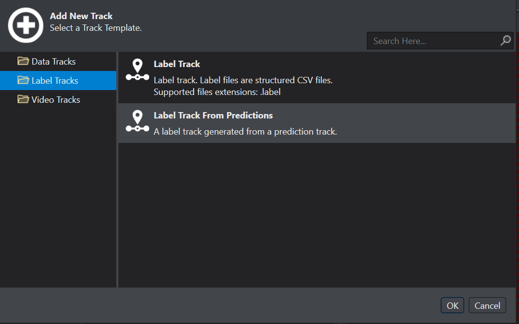
The Generate label track from predictions window appears.

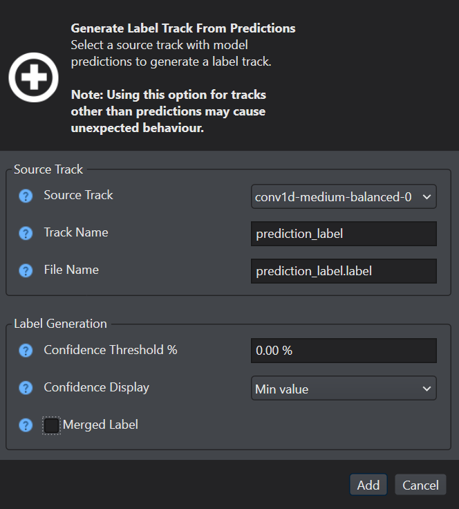
13. Configure the following parameters-

    • In Source Track, select the model that should be used to generate prediction label track.

    • In Track Name, enter the name of the prediction label track.

    • In File Name, enter the name of the prediction label file.

    • In Confidence Threshold %, enter the confidence percentage value as zero.

    • In Confidence Display, select the confidence display type.

    • In Merged Label, disable the checkbox to view the separated labels.

14. Click Add to confirm. A new label track with the specified track name is created. The track contains the labels generated by the model.
    

    
    

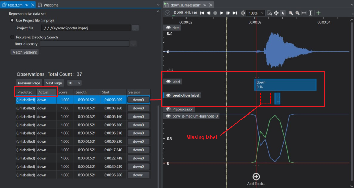
On comparing the actual and predicted label tracks, we can see that the down event was predicted as unlabelled by model. This helps us in visualizing the predictions which can be used to improve the model further.